Defining the user requirements for the food security use case

Food security, especially in a changing Earth environment, is one of the most challenging issues of this century. Population growth, increased food consumption, and the challenges of climate change will extend over the next decades. To deal with these, both regional and global measures are necessary. There is a need to increase biomass production which means to increase the yield in a sustainable way. It is important to minimize the risks of yield loss even under more extreme environmental conditions, while making sure not to deplete or damage the available resources.

Irrigation, as one of the most important measures for food production, requires reliable water resources in the area that is being farmed, either from ground water or surface water. Irrigation planning and choosing the right measures at the right time, requires detailed and reliable information on status and prospects of water availability.

One of our first jobs within the Extreme Earth Project is to define the user requirements. To start with this, we have to ask us the following questions:

1. Who are the users?

   Users can come from numerous areas with different background: For course, the most obvious users are the farmers themselves, or better representatives from large agricultural companies. But of course, also irrigation companies or consulting agencies might be very interested in the information we will gain through this project. Maybe the most important users are the stakeholders or decision makers from communal, federal and national governments or even the EU authorities. We did some research to find the according key persons of each category and invited them to our first User’s Workshop that we organised in March in Munich.

2. What are their requirements or their needs in terms of food security?

   After intense discussions with a group of potential demo users on our User’s workshop we also created a questionnaire to identify the additional user’s needs. The evaluation of this questionnaire will give us more information about technical requirements like resolution, format and accessibility of the final product, as well as thematic requirements like areas of interest and main crops.

3. Why do we focus on irrigation?

   To sustain global food security, two practices are of high importance: irrigation and fertilization. Fertilisation is a bio-chemical process that can be controlled and optimized through agricultural management. It relies mainly on industrial goods, and the resources for it can be transported if the necessary infrastructure is available.

   Water availability is – in contrast to fertilisation – a highly variable and often uncertain variable. Limited water availability can be an issue for many farmers, industries and governments. A large portion of the world’s fresh water is linked to snowfall, snow storage and seasonal release of the water. All these components are subject to increased variability due to climate change and this might result in an increase in extreme events.

   With the use of the Earth Observation data, modelling and in-situ measurements of the snow cover, all necessary information regarding water availability can be obtained – especially now using sophisticated deep learning techniques to handle the large data volume of the Copernicus archive. With this approach VISTA will be able to combine for example seasonal information about water storage in the Alps, with the highly dynamic water demand in agricultural areas such as the Danube area and give large scale recommendations for private farmers, but also for national governments about sustainable water usage.

How ExtremeEarth Brings Large-scale AI to the Earth Observation Community with Hopsworks, the Data-intensive AI Platform

In recent years, unprecedented volumes of data are generated in various domains. Copernicus, a European Union flagship programme, produces more than three petabytes(PB) of Earth Observation (EO) data annually from Sentinel satellites. This data is made readily available to researchers that are using it, among other things, to develop Artificial Intelligence (AI) algorithms in particular using Deep Learning (DL) techniques that are suitable for Big Data. One of the greatest challenges that researchers face however, is the lack of tools that can help them unlock the potential of this data deluge and develop predictive and classification AI models.

ExtremeEarth is an EU-funded project that aims to develop use-cases that demonstrate how researchers can apply Deep Learning in order to make use of Copernicus data in the various EU Thematic Exploitation Platforms (TEPs). A main differentiator of ExtremeEarth to other such projects is the use of Hopsworks, a Data-Intensive AI software platform for scalable Deep Learning. Hopsworks is being extended as part of ExtremeEarth to bring specialized AI tools for EO data and the EO data community in general.

Hopsworks, Earth Observation Data and AI in one Platform

Hopsworks is a Data-Intensive AI platform which brings a collaborative data science environment to researchers who need a horizontally scalable solution to developing AI models using Deep Learning. Collaborative means that users of the platform get access to different workspaces, called projects, where they can share data and programs with their colleagues, hence improving collaboration and increasing productivity. The Python programming language has become the lingua franca amongst data scientists and Hopsworks is a Python-first platform, as it provides all the tools needed to get started programming with Python and Big Data. Hopsworks integrates with Apache Spark and PySpark, a popular distributed processing framework.

Hopsworks brings to the Copernicus program and the EO data community essential features required for developing aI applications at scale, such as distributed Deep Learning with Graphics Processing Units (GPUs) on multiple servers, as demanded by the Copernicus volumes of data. Hopsworks provides services that facilitate conducting Deep Learning experiments, all the way from doing feature engineering with the Feature Store, to developing Deep Learning models with the Experiments and Models services that allow them to manage and monitor Deep Learning artifacts such as experiments, models and automated code-versioning and much more . Hopsworks storage and metadata layer is built on top of HopsFS, the award-winning highly scalable distributed file system, which enables Hopsworks to meet the extreme storage and computational demands of the ExtremeEarth project.

Hopsworks brings horizontally scalable Deep Learning for EO data close to where the data lives, as it can be deployed on Data and Information Access Services (DIAS). The latter provides centralised access to Copernicus data and information which combined with the AI for EO data capabilities that Hopsworks brings, an unparalleled data science environment is made available to researchers and data scientists of the EO data community.

Challenges of Deep Learning with EO Data

Recent years have witnessed the performance leaps of Deep Learning (DL) models thanks to the availability of big datasets (e.g. ImageNet) and the improvement of computation capabilities (e.g., GPUs and cloud environments). Hence, with the massive amount of data coming from earth observation satellites such as the Sentinel constellation, DL models can be used for a variety of EO-related tasks. Examples of these tasks are sea-ice classification, monitoring of water flows, and calculating vegetation indices.

However, together with the performance gains comes many challenges for applying DL to EO tasks, including, but not limited to:

• Labeled datasets for training: While collecting raw Synthetic-Aperture Radar (SAR) images from the satellites is one thing, labeling those images to make them suitable for supervised DL is yet a time consuming task. Should we seek help from unsupervised or semi-supervised learning approaches to eliminate the need for labeled datasets? Or should we start building tools to make annotating the datasets easier?
• Interpretable and Human-understandable models or EO tasks: Given enough labeled data, we can probably build a model with satisfactory performance. But how can we justify the reasons behind why the model makes certain predictions given certain inputs? While we can extract the intermediate predictions for given outputs, can we reach interpretations that can be better understood by humans?
• Management of very large datasets: Managing terabytes (TB) of data that can still fit into a single machine is one thing, but managing petabytes (PB) of data that requires distributed storage and provides a good service for the DL algorithms so as not to slow down the training and serving process is a totally different challenge. To further complicate the management, what about partial failures in the distributed file system? How shall we handle them?
• Heterogeneous data sources and modalities (e.g., SAR images from satellites, sensor readings from ground weather stations): How can we build models that effectively use multi-modalities? For example, how can we utilize the geo-location information in an image classification model?
• DL architectures and learning algorithms for spectral, spatial, and temporal data: While we might be able to perform preprocessing and design model architectures for RGB image classification, how do these apply to SAR images? Can we use the same model architectures? How to extract useful information from multi-spectral images?
• Training and fine-tuning (hyperparameter optimizations) of DL models: Hyperparameters are those parameters of the training process (e.g., the learning rate of the optimizer, or the size of the convolution windows) that should be manually set before training. How can we effectively train models and tune the hyperparameters? Should we change the code manually? Or can we use frameworks to provide some kind of automation?
• The real time requirements for serving DL models: Once the training is done, we want to use our trained model to predict outcomes based on the newly observed data. Often these predictions have to be made in real-time or near-real-time to make quick decisions. For example, we want to update the ice charts of the shipping routes every hour. How to serve our DL models online to meet these real-time requirements?

Deep Learning Pipelines for EO Data with Hopsworks

A Data Science application in the domain of Big Data typically consists of a set of stages that form a Deep Learning pipeline. ُThis pipeline is responsible for managing the lifecycle of data that comes into the platform and is to be used for developing machine learning models. In the EO data domain in particular, these pipelines need to scale to the petabyte-scale data that is available within the Copernicus program. Hopsworks provides data scientists with all the required tools to build and orchestrate each stage of the pipeline, depicted in the following diagram.

In detail, a typical Deep Learning pipeline would consist of:

• Data Ingestion: The first step is to collect and insert data into the AI platform where the pipeline is to be run. A great variety of data sources can be used such as Internet of Things (IoT) devices, web-service APIs etc. In ExtremeEarth, the data typically resides on the DIAS which can be directly accessed from Hopsworks.
• Data Validation: Tools such as Apache Spark that can cope with Big Data are typically employed to validate incoming data that is to be used in later stages. For example data might need to be parsed and cleaned up from duplicate or missing values or a simple transformation of an alphanumeric field to a numeric one might be needed.
• Feature Engineering: Before making use of the validated data to develop DL models, the features that will be used to develop such models need to be defined, computed and persisted. Hopsworks Feature Store is the service that data engineers and data scientists use for such tasks, as it provides rich APIs, scalability and elasticity to cope with varying data volumes and complex data types and relations. For example users can create groups of features or compute new features such as aggregations of existing ones.
• Model development (Training): Data scientists can greatly benefit from a rich experiment API provided by Hopsworks to run their machine learning code, whether it be TensorFlow, Keras, PyTorch or another framework with a Python API. In addition, Hopsworks manages GPU allocation across the entire cluster and facilitates distributed training which involves making use of multiple machines with multiple GPUs per machine in order to train bigger models and faster.
• Model Serving & Monitoring: Typically the output of the previous stage is a DL model. To make use of it, users can submit inference requests by using the Hopsworks built-in elastic model serving infrastructure for TensorFlow and scikit-learn, two popular machine learning frameworks. Models can also be exported in the previous pipeline and downloaded from Hopsworks directly to be embedded into external applications, such as iceberg detection and water availability detection in food crops. Hopsworks also provides infrastructure for model monitoring, that is continuously monitoring the requests being submitted to the model and its responses and users can then apply their own business logic on which actions to take depending on how the monitoring metrics output changes over time.

Example Use Case: Iceberg Classification with Hopsworks

Drifting icebergs pose major threats to the safety of navigation in areas where icebergs might appear, e.g., the Northern Sea Route and North-West Passage. Currently, domain experts manually conduct what is known as an “ice chart” on a daily basis, and send it to ships and vessels. This is a time-consuming and repetitive task, and automating it using DL models for iceberg classification would result in generation of more accurate and more frequent ice charts, which in turn leads to safer navigation in concerned routes.

Iceberg classification is concerned with telling whether a given SAR image patch contains an iceberg or not. Details of the classification depends on the dataset that will be used. For example, given the Statoil/C-CORE Iceberg Classifier Challenge dataset, the main task is to train a DL model that can predict whether an image contains a ship or an iceberg (binary classification).

The steps we took to develop and serve the model were the following:

• First step is preprocessing. We read the data which is stored in JSON format and create a new feature which is the average of the satellite image bands.
• Second step is inserting the data into the Feature Store which provides APIs for managing feature groups and creating training and test datasets. In this case, we created the training and test datasets in TFRecord format after scaling the images as we are using TensorFlow for training.
• Third step is building and training our DL model on Hopsworks. Since the dataset is not very complicated and we have a binary classification task, using a DL model that is very similar to LeNet-5 yields 87% accuracy on the validation set after 20 epochs of training which takes 60 seconds to train on a Nvidia GTX1080. This step also includes hyperparameter tuning. Ablation studies, in which we remove different components (e.g., different convolutional layers, or dataset features) can also be employed to gain more insights about the model. Hopsworks provides efficient and easy support for hyperparameter tuning and ablation studies through a Python-based framework called Maggy. Finally, to further increase the training speed, the distributed training strategy provided in Hopworks can be used.

The final step is to export and serve the model. Model is exported and saved into the Hopsworks “Models” dataset. Then we use the Hopsworks elastic model serving infrastructure to host TensorFlow serving which can scale with the number of inference requests.

Conclusion

In this blog post we described how the ExtremeEarth project brings new tools and capabilities with Hopsworks to the EO data community and the Copernicus program. We also showed how we have developed a practical use case by using Copernicus data and Hopsworks. We keep developing Hopsworks to make it even more akin to the tools and processes used by researchers across the entire EO community and we continue development of our use cases with more sophisticated models using even more advanced distributed Deep Learning training techniques.

Regular Monitoring of Agricultural Areas using Sentinel 2 Image Time Series and Deep Learning Techniques

With the advent of the Copernicus European programs, completely full, open and free remote sensing data are constantly acquired at a global scale. These data are extremely useful for regularly monitoring the Earth’s surface. In particular, the multispectral high-resolution optical images acquired by Sentinel 2 are suited for the monitoring of agricultural areas, which need to be frequently updated since cultivations change their spectral and textural appearance according to their crop type growth cycle. Sentinel 2 is characterized by specific bands in the Red-Edge spectral range dedicated to the study of vegetation, which allow the characterization of the phenological parameters of different crop types. In this context, ExtremeEarth aims to define a system architecture able to fully exploit the long time series of Sentinel 2 images to perform accurate and regular monitoring of agricultural areas at large scale.

This peculiar classification problem requires the definition of a multitemporal approach that accurately characterizes the different crop types, which have their own phenological characteristics and development times. Instead of using a pre-trained network, ad-hoc deep network architecture tailored to the specific spatial, temporal and spectral nature of dense time series of Sentinel 2 will be defined. Given the complexity of the considered problem, an automatic system architecture based on recurrent deep neural networks will be considered by focusing the attention on the Long Short Term Memory (LSTM). These deep learning models are able to capture the temporal correlation of sequential data, by storing an unlimited amount of evidence and make decisions in that actual temporal context.

The first experimental analysis will be carried out on the whole Danube catchment, which is characterized by considerably extent (801.463 km²) and heterogenous environmental conditions. At such large scale, many challenges have to be addressed. First, the deep learning architecture has to handle the fact that the spectral signatures of the land-cover classes are characterized by high spatial variability. Hence, due to physical factors (e.g., acquisition conditions, soil properties) the same crop types may present different spectral properties in the different region of the Danube Catchment. Then, it is important to take into account the presence of highly unbalanced classes as well as to properly model the high inter-class and low-intraclass variance to guarantee a consistent classification product. Moreover, for the reliable training of deep networks, millions of annotated samples are required. While in computer vision many large databases of labelled images are available, in remote sensing it is not feasible to collect in-situ data at such a scale. Hence, a large training database of "weak" labelled samples will be defined in an unsupervised and automatic way.

Example of crop type map that will be produced for the whole Danube Catchment. The 17 crop types that will be identified are reported.

The system will generate crop type and crop boundaries maps at 10m of spatial resolution, the highest resolution achieved by Sentinel 2. The crop type maps will be characterized by 17 different main cultivations, namely, Grassland, Forage, Oat, Potato, Beet, Spring Wheat, Winter Wheat, Permanent Plantations, Maize, Legumes, Rapeseed, Rye, Spring Barley, Winter barley, Soy, and Flowering legumes. The preliminary test will be performed using the time series of Sentinel 2 images acquired in 2018. To validate the results obtained the 2018 European Land Use and Coverage Area Frame Survey (LUCAS) database will be used. The LUCAS survey, coordinated by the Statistical Office of the European Commission (Eurostat), aims to collect harmonized data land cover/land use, agro-environmental and soil data by field observation of geographically referenced points.

New sea ice and iceberg datasets created within the polar use case

Within ExtremeEarth, the polar use case will develop automatic methods for classifying sea ice which can be used in the production of ice charts. This will streamline existing ice charting workflows and allow ice analysts to focus on products which are currently out of the reach of machine learning techniques.

In this blogpost we will focus on an important aspect of the development of automatic methods; the training data that is used in the training of the algorithms. Supervised learning of machines requires labelled data for training the machines to be well-performing decision-makers.

New sea ice datasets

These new sea ice datasets are publicly available with the DOI. The plan is to use these as common datasets for the project, being able to compare methods on the same data. The three datasets represent each of the three use cases within the polar use case: Ice edge, ice types, and icebergs:

1. The ice edge dataset is a binary dataset with the two classes ice and sea.
2. The icetypes dataset contains segmented images, where each segment contains one among more specific ice types, or sea.
3. The iceberg dataset contains outlines of all icebergs observed within one Sentinel-2 image.

All images used in all datasets are over the same geographical area in the seas east of Greenland, and are acquired in the year 2018. The two first datasets each consist of twelve images for each month in 2018 and for the third dataset we have Sentinel-2 image from March 2018.

Why do we need labelled data?

Labelled data are made by assigning labels to data entries. The sea ice classification and detection algorithms we are working with use satellite images as input data. That could for instance be radar images from the synthetic aperture radar Sentinel-1, or an optical image from the Sentinel-2 optical satellite. A satellite image over the Arctic areas may contain different types of sea ice, open water, and also pieces of land. Thus the image may contain multiple different surface type labels.

A closer look on the iceberg dataset with the Sentinel-2 image in background. The red outlines are marked icebergs. The blue lines are the segment outlines drawn for the March image in the ice type dataset.

A majority of the automatic deep learning algorithms need a ground truth to compare the input data with during training. The machine needs to see the connection between different kinds of image features and the connected label name. When it has seen many such connections, it may be able to make a good decision on what it sees in a new image.

Distributed geospatial analytics over linked data in ExtremeEarth

The information produced by the deep learning pipelines of the ExtremeEarth project will contain useful knowledge that the end users should access. This information will be transformed to linked RDF data over a familiar vocabulary for the users, in the form of ontological classes and properties, and will be interlinked with other useful datasets. A system that will store and query all these massive linked spatial RDF datasets on the HOPS platform is under development as part of the ExtremeEarth. This system will provide the user with the capability to explore the datasets, obtain useful information and perform rich spatial analytics using the GeoSPARQL query language. The system is built using the popular distributed in-memory processing framework Spark, and its extension GeoSpark for spatial partitioning, indexing and processing, and it works by translating an input GeoSPARQL query into a series of Spark jobs.

Apart from the spatial partitioning of the geometries contained in the dataset, the system also employs advanced partitioning techniques for the thematic RDF data, aiming to provide efficient execution by minimizing data transfer across the network, and also minimize the amount of data that need to be accessed for each query. The system has already been tested in the HOPS platform with a spatial RDF dataset of more than 1 billion triples and 100 million complex geometries, which already exceeds the data size that centralized state of the art geospatial RDF stores can handle in a single server with up to 128 GB of memory.

Several improvements are currently under development, including specialized compression techniques like dictionary or prefix-based encoding for the thematic RDF data, and an efficient cost-based query optimizer that will take into consideration both thematic and spatial query selectivity in order to decide about the execution order of the query operators and the usage of the spatial access methods of the underlying data (partitioning and indexing schemes).

JedAI: An open-source library for state-of-the-art large scale data integration

The Java gEneric DAta Integration system (JedAI) constitutes an open source, high scalability toolkit that offers out-of-the-box solutions for any data integration task, e.g., Record Linkage, Entity Resolution and Link Discovery. At its core lies a set of domain-independent, state-of-the-art techniques that apply to data of any structuredness: from the structured data of relational databases and CSV files to the semi-structured data of SPARQL endpoints and RDF dumps and to unstructured (i.e., free text) Web data. Any combination of these data types is also possible.

Before ExtremeEarth, JedAI’s latest release, version 2.0, implemented a single end-to-end workflow that was based on batch, schema-agnostic blocking techniques [1].

The batch, blocking-based end-to-end workflow of JedAI.

This workflow was implemented by JedAI-core, the back-end of the system, while JedAI-gui provided a front-end that is suitable for both expert and lay users. JedAI-gui actually is a desktop application with a wizard-like interface that allows users to select among the available methods per workflow step so as to form end-to-end pipelines. The relation of the two modules is depicted in the following figure.

The system architecture of JedAI version 2.

In the context of ExtremeEarth, we upgraded JedAI to versions 2.1 [2] and 3.0 [3], improving it substantially in all respects.

More specifically, its back-end has been enriched with the following three end-to-end workflows:

1. A batch, schema-based workflow that is based on string similarity joins, as shown in the figure. Compared to the schema-agnostic, blocking-based workflow, it offers lower effectiveness for much higher efficiency, provided that there are reliable attributes (i.e., predicates) for matching entities according to the similarity of their values (e.g., the title of publications in bibliographic datasets).

   

   The batch, schema/join-based end-to-end workflow of JedAI.

2. A progressive schema-agnostic workflow that extends the corresponding batch workflow in Figure 1 with a Prioritization step, as shown in Figure 4. The goal of this step is to schedule the processing of entities, blocks or comparisons according to the likelihood that they involve duplicates. This enables JedAI to operate in a pay-as-you-go fashion that detects matches early on and terminates the entire processing on-time, i.e., when the likelihood of detecting additional duplicates is negligible. As a result, we can minimize the run-time of applications that can operate on partial results or have access to limited computational resources.

   

   The budget-agnostic (progressive), blocking-based end-to-end workflow of JedAI. The shaded workflow steps are optional, as some progressive methods can be applied directly to the input entities, while self-loops indicate steps that can be repeated, using a different method each time.

3. A progressive schema-based workflow that involves the same steps as its budget-agnostic (batch) counterpart in Figure 3. The only difference is that Top-k Similarity Join is used for detecting the candidate matches in non-increasing order of estimated similarity – either globally, across the entire dataset, or locally, for individual entities.

Additionally, JedAI version 3.0 adapts all algorithms of JedAI-core to the Apache Spark framework and implements them in Scala. Through Apache Spark’s massive parallelization, JedAI is able to minimize the run-time of any end-to-end ER workflow, a goal that is in line with ExtremeEarth’s target to tackle huge volumes of data. The code is available here.

Overall, these new features equip JedAI with support for three-dimensional Entity Resolution, as it is defined in Figure 5. The first dimension corresponds to schema-awareness, distinguishing between schema-based and schema-agnostic workflows. The second dimension corresponds to budget-awareness, distinguishing between budget-agnostic (i.e., batch) and budget-aware (i.e., progressive) workflows. The third dimension corresponds to the execution mode, which distinguishes between serial and massively parallel processing. JedAI supports all possible combinations of the three dimensions, which is a unique feature across all open-source data integration tools, as they are typically restricted to schema-based, batch workflows (grey area in the figure).

The solution space of the end-to-end ER pipelines that can be constructed by JedAI version 3.

Another advantage of JedAI is its extended coverage of the state-of-the-art techniques for Entity Resolution. Every workflow step in all end-to-end workflows conveys a series of state-of-the-art approaches. Thus, unlike the other open-source tools, which typically offer a limited number of methods, JedAI enables users to build millions of different end-to-end pipelines.

JedAI’s version 3 also improves its user interface in three ways:

1. By adding a command line interface that offers the same functionalities as the desktop application.

2. Through a Python wrapper that is based on pyjnius, JedAI can be seamlessly used in a Jupyter Notebook.

3. Through a novel Web application with a wizard-like interface that provides a unified access to local execution (on a single machine) and to remote execution (over a cluster through Apache Livy). This Web application can be easily deployed through a Docker image. A video demonstrating its use and capabilities is available here.

The new system architecture in Figure 6 shows how all these improvements have been integrated into JedAI version 3. A technical report that analytically describes all components and evaluates their performance over a series of established datasets is available here.

The system architecture for JedAI version 3.

At the moment, we are also working on extending JedAI with techniques that are suitable for geospatial interlinking. We are adding support for all topological relations of the DE-9IM model, such as contains, crosses, covers and disjoint. To this end, we have integrated the state-of-the-art blocking-based methods of Silk [4] and Limes [5] (namely Radon [6]) into JedAI. We have also developed new techniques that improved the existing ones by facilitating their adaptation to the Apache Spark framework. We are performing thorough experimental analysis to verify the high scalability of our novel techniques, demonstrating that they are capable of handling tens of millions of geometries.

References

[1] George Papadakis, Leonidas Tsekouras, Emmanouil Thanos, George Giannakopoulos, Themis Palpanas, Manolis Koubarakis. "The return of JedAI: End-to-End Entity Resolution for Structured and Semi-Structured Data". Proc. VLDB Endow. 11(12): 1950-1953 (2018)

[2] George Papadakis, Leonidas Tsekouras, Emmanouil Thanos, George Giannakopoulos, Themis Palpanas, Manolis Koubarakis. "Domain- and Structure-Agnostic End-to-End Entity Resolution with JedAI". SIGMOD Rec. 48(4): 30-36 (2019)

[3] George Papadakis, Leonidas Tsekouras, Emmanouil Thanos, Nikiforos Pittaras, Giovanni Simonini, Dimitrios Skoutas, Paul Isaris, George Giannakopoulos, Themis Palpanas, Manolis Koubarakis. "JedAI3: beyond batch, blocking-based Entity Resolution". EDBT 2020: 603-606

[4] Panayiotis Smeros, Manolis Koubarakis. "Discovering Spatial and Temporal Links among RDF Data". LDOW@WWW 2016

[5] Axel-Cyrille Ngonga Ngomo, Sören Auer. "LIMES - A Time-Efficient Approach for Large-Scale Link Discovery on the Web of Data". IJCAI 2011: 2312-2317

[6] Mohamed Ahmed Sherif, Kevin Dreßler, Panayiotis Smeros, Axel-Cyrille Ngonga Ngomo. "Radon - Rapid Discovery of Topological Relations". AAAI 2017: 175-181

AI Software Architecture for Copernicus Data with Hopsworks

TLDR: Hopsworks, the data-intensive AI platform with a feature store, brings support for scale-out AI with Copernicus data and the H2020 ExtremeEarth project. Hopsworks is integrated with the Polar and FoodSecurity Thematic Exploitation Platforms (TEPs) on the CREODIAS infrastructure. Two use cases, polar and food security, have been developed by making use of the scale-out distributed deep learning support of Hopsworks and the PBs of data made available by CREODIAS and processed by Hopsworks and the TEPs .

This article is based on the paper “The ExtremeEarth software Architecture for Copernicus Earth Observation Data” included in the Proceedings of the 2021 conference on Big Data from Space (BiDS 2021) [1].

Introduction

In recent years, unprecedented volumes of data are being generated in various domains. Copernicus, a European Union flagship programme, produces more than three petabytes (PB) of Earth Observation (EO) data annually from Sentinel satellites [2]. However, current AI architectures making use of deep learning in remote sensing are struggling to scale in order to fully utilize the abundance of data.

ExtremeEarth is an EU-funded project that aims to develop use-cases that demonstrate how researchers can apply deep learning in order to make use of Copernicus data in the various European Space Agency (ESA) TEPs. A main differentiator of ExtremeEarth to other such projects is the use of Hopsworks, a Data-Intensive AI software platform with a Feature Store and tooling for horizontally scale-out learning. Hopsworks has successfully been extended as part of ExtremeEarth project to bring specialized AI tools to the EO data community with 2 use cases already developed on the platform with more to come in the near future.

Bringing together a number of cutting edge technologies, which deal from storing extremely large volumes of data all the way to performing scalable machine learning and deep learning algorithms in a distributed manner, and having them operate over the same infrastructure poses some unprecedented challenges. These challenges include, in particular, integration of ESA TEPs and Data and Information Access Service (DIAS) platforms with a data platform (Hopsworks) that enables scalable data processing, machine learning and deep learning on Copernicus data; development of very large training datasets for deep learning architectures targeting the classification of Sentinel images.

In this blog post, we describe both the software architecture of the ExtremeEarth project with Hopsworks as its AI platform centerpiece and the integration of Hopsworks with the other services and platforms of ExtremeEarth that make up for a complete AI with EO data experience.

AI with Copernicus data - Software Architecture

There are several components that comprise the overall architecture with the main ones being the following.

Hopsworks. An open-source data-intensive AI platform with a feature store. Hopsworks can scale to the petabytes of data required by the ExtremeEarth project and provides tooling to build horizontally scalable end-to-end machine learning and deep learning pipelines. Data engineers and data scientists utilize Hopsworks’ client SDKs that facilitate AI data management, machine learning experiments, and productionizing serving of machine learning models.

Thematic Exploitation Platforms (TEPs). These are collaborative, virtual work environments providing access to EO data and the tools, processors, and Information and Communication Technology (ICT) resources required to work with various themes, through one coherent interface. TEPs address coastal, forestry, hydrology, geohazards, polar, urban themes, and food security themes. ExtremeEarth in particular is concerned with the polar and food security TEPs where the use cases also stem from. These use cases include building machine learning models for sea ice classification to improve maritime traffic as well as food crops and irrigation classification.

Data and Information Access Service (DIAS). To facilitate and standardize access to data, the European Commission has funded the deployment of five cloud-based platforms. They provide centralized access to Copernicus data and information, as well as to processing tools. These platforms are known as the DIAS, or Data and Information Access Services [2]. ExtremeEarth software architecture is built on CREODIAS, a Cloud infrastructure platform adapted to the processing of big amounts of EO data, including an EO data storage cluster and a dedicated Infrastructure-as-a-Service (IaaS) Cloud infrastructure for the platform’s users. The EO data repository contains Sentinel-1, 2, 3, and 5-P, Landsat-5, 7, 8, Envisat, and many Copernicus Services data.

Figure 1: ExtremeEarth software architecture.

Figure 1 provides a high-level overview of the integration of the different components with each other. The components can be classified into four main categories(layers):

• Product layer. The product layer provides a collaborative virtual work environment, through TEPs, that operates in the cloud and enables access to the products, tools, and relevant EO, and non-EO data.
• Processing layer. This layer provides the Hopsworks data-intensive Artificial Intelligence (AI) platform. Hopsworks is installed within the CREODIAS OpenStack cloud infrastructure and operates alongside the TEPs. Also, Hopsworks has direct access to the data layer and the different data products provided by the TEPs.
• Data layer. The data layer offers a cloud-based platform that facilitates and standardizes access to EO data through a Data and Information Access Service (DIAS). It also provides centralized access to Copernicus data and information, as well as to processing tools. TEPs are installed and run on a DIAS infrastructure, which in the case of ExtremeEarth is the CREODIAS.
• Physical layer. It contains the cloud environment’s compute, storage, networking resources, and hardware infrastructures.

To provide a coherent environment for AI with EO data to application users and data scientists, the goal of the architecture presented here is to make most components transparent and simplify developer access by using well-defined APIs while making use of commonly used interfaces such as RESTful API. As a result, a key part of the overall architecture is how these different components can be integrated to provide a coherent whole. The APIs used for the full integration of the ExtremeEarth components via the inter-layer interfaces of the software platform are described below and also are illustrated in Figure 1:

1. Raw EO data. DIASes and CREODIAS in particular, provide Copernicus data access which includes the downstream of Copernicus data as it is generated by satellites. At an infrastructure level, this data is persisted at an object store with an S3 object interface, managed by CREODIAS.
2. Pre-processed data. TEPs provide the developers of the deep learning pipelines with pre-processed EO data which forms the basis for creating training and testing datasets. Developers of the deep learning pipeline can also define and execute their own pre-processing, if the pre-processed data is not already available.
3. Object storage. CREODIAS provides object storage used for storing data produced and consumed by the TEPs services and applications. In ExtremeEarth, this object store is used primarily for storing training data required by the Polar and Food Security use cases. This training data is provided as input to the deep learning pipelines.
4. EO Data Hub Catalog. This service is provided and managed by CREODIAS. It provides various protocols including OGC WFS and a REST API as interfaces to the EO data.
5. TEP-Hopsworks EO data access. Users can directly access raw EO data from their applications running on Hopsworks. Multiple methods, e.g., object data access API (SWIFT/S3), filesystem interface, etc., are provided for accessing Copernicus and other EO-data available on CREODIAS.
6. TEP-Hopsworks infrastructure Integration. Hopsworks and both the Polar and Food Security TEPs are installed and operated on CREODIAS and its administrative tools enable TEPs to spawn and manage virtual machines and storage by using CloudFerro [3] which provides an OpenStack-based cloud platform to TEPs. Hopsworks is then installed in this platform and it can access compute and storage resources provided by the TEPs.
7. TEP-Hopsworks API integration. Hopsworks is provided within the TEP environment as a separate application and is mainly used as a development platform for the deep learning pipelines and applications of the Polar and Food Security use cases. These applications are exposed in the form of processors to the TEP users. Practically, a processor is a TEP abstraction that uses machine learning models that have previously been developed by the data scientists of the ExtremeEarth use cases in Hopsworks.
8. Hopsworks-TEPs datasets. TEPs provide users with access to data to be served as input to processors from various sources. Such sources include the data provided by CREODIAS and external services that the TEP can connect to. The pre-processed data is stored in an object storage provided by CREODIAS, thus made available to Hopsworks users by exchanging authentication information. Hopsworks users can also upload their own data to be used for training or serving. Hopsworks provides a REST API for clients to work with model serving, and authentication is done in the form of API keys managed by Hopsworks on a per user basis. These keys can therefore be used by external clients to authenticate against the Hopsworks REST API. There are two ways by which the trained model can be served via the TEP: (i) The model can be exported from Hopsworks and be embedded into the TEP processor. (ii) The model can be served online on Hopsworks and a processor on the TEP submits inference requests to the model serving instance on Hopsworks and returns the results. In method (i), once the machine learning model is developed, it can then be transferred from Hopsworks to the Polar TEP by using the Hopsworks REST API and Python SDK. TEP users can integrate the Hopsworks Python SDK into the processor workflow to further automate the machine learning pipeline lifecycle. In method (ii), the TEP is able to submit inference requests to the model being served by the online model serving infrastructure run on Kubernetes and hosted on Hopsworks. Figure 2 illustrates this approach for the Polar use case.
9. Linked Data tools. Linked data applications are deployed as Hopsworks jobs using Apache Spark. A data scientist can work with big geospatial data using ontologies and submit GeoSPARSQL queries using tools developed and extended within ExtremeEarth, namely GeoTriples [4], Strabo2, JedAI-Spatial, and Semagrow.

Figure 2: ExtremeEarth software architecture for the Polar Use Case.

Application users that interact with the TEPs effectively are the users of the AI products generated by the machine learning and deep learning pipelines developed by the data scientists in Hopsworks. Previously we described the integration of the various components. Figure 3 depicts the flow of events within this architecture:

1. EO data scientists log in to Hopsworks.
2. Read and pre-process raw EO data in Hopsworks, TEP or in the local machine.
3. Create training datasets based on the intermediate pre-processed data.
4. Develop deep learning pipelines.
5. Perform linked data transformation, interlinking, and storage.
6. Log in to the Polar or Food Security TEP applications.
7. Select Hopsworks as the TEP processor. The processor starts the model serving in Hopsworks via the REST API. The processor also downloads the model from Hopsworks via the REST API and serving is done within the TEP application.
8. Submit federated queries with Semagrow and use the semantic catalogue built into Hopsworks.

Figure 3: ExtremeEarth software architecture flow of events

Conclusion

In this blog, we have shown how Hopsworks has been integrated with various services and platforms in order to extract knowledge from AI and build AI applications using Copernicus and Earth Observation data. Already two use cases, sea ice classification (PolarTEP) and crop type mapping and classification (Food Security TEP ), have been developed using the aforementioned architecture by using the PBs of data made available by the Copernicus programme and infrastructure.

If you would like to try it out yourself, make sure to register an account at https://hopsworks.polartep.io/hopsworks. You can also follow hopsworks on GitHub and Twitter.

References

[1] Proceedings of the 2021 conference on Big Data from Space 18-20 May 2021

[2] Copernicus General Overview

[3] Data and Information Access Services

[4] GeoTriples Spark

Processing large Earth Observation Datasets using the Hopsworks platform

In recent years, remote sensing images have become more and more available thanks to open data policies and new satellite constellations with a short revisit time. This is the case of the European Copernicus programs, where open and free data are acquired over the entire globe providing 12 terabytes daily. In order to exploit such big data sources, ad-hoc platforms that can effectively handle large amounts of data are required. In the context of the Extreme Earth project, this role is filled by Hopsworks, a Data-Intensive AI software platform for scalable Deep Learning.

The aim of this post is to provide an overview of how such a platform can be used to process a large Earth Observation (EO) dataset (i.e., a time-series of images) and how the Hopsworks platform can be used to train deep learning models for such tasks. To this end, an implementation in Python is provided in a Jupyter notebook. These examples are based on the use of the Hopsworks web interface.

Data Storage

Hopsworks stores files using a custom distribution of the Hadoop Distributed File System defined as HopsFile System (HopsFS) based on distributed metadata service built on a NewSQL database. The files can be accessed using the Dataset tab which allows for the navigation through files and directories.

Figure 1: Example of the Dataset tab

In this example, we are considering the processing of multiple images. From the Dataset tab it is possible to create a new dataset as a new empty folder that can be filled with the images by a direct upload using the interface. Another option (which is more suitable for large datasets and processing) is to transfer the data from another platform (e.g., Food Security TEP) using a script that downloads the images and then transfers them on the HopsFS.

Data Access and Processing

In order to process the data, first they have to be moved from HopsFS to the local machine. This can be done with the hops library which provides functionalities to access the HopsFS. In this example, we consider a dataset composed of 5 time series, each one corresponding to a Sentinel-2 tile.

The access to the data is straightforward and requires the user to copy the data on the local file system while all the rest of the implementation requires no changes. The hdfs.copy_to_local copy the images on the local file system which can now be loaded to be processed.

The script iterates over each tile, loading each image individually for processing. After each image has been processed, it is copied back to the HopsFS using the hdfs.copy_to_hdfs function.

Model Training

The Hopsworks platform is designed specifically for the development and operation of machine learning models with a focus on deep learning. In detail, the platform provides the Experiments API which allows the user to train different models, on different frameworks (e.g., Tensorflow, PyTorch). A relevant function of the Experiment API is the Distributed Training which allows for the use of multiple machines/GPUs to train the model while being almost completely transparent to the user implementation. Indeed, to run a distributed training using the Experiment API it is sufficient to provide the training code inside a wrapper function. Such functionalities are based on PySpark.

Here we provide an example of the training of a model for crop type classification using Sentinel-2 time series. To this end, we use the TimeSen2Crop dataset which is freely available. The dataset can be uploaded to the Hopsworks and accessed as described in the previous section.

To launch such training in a distributed training environment, the function is simply given as input to the Experiment API which will handle the distribution of the training tasks to the multiple machines without any additional code required to the user.

Launch the Experiment

To launch the Experiments (i.e., the training process) in a distributed fashion, first we need to define the distributed environment in terms of workers, GPUs per worker and available memory and configure the PySpark kernel. This can be done from the Jupyter tab selecting the Experiments configuration:

Figure 2: Example of Experiments configuration for distributed training

After having started the Jupyter, the distributed training can be launched by starting the corresponding notebook.

Monitoring the Experiment

Training deep learning models is often a lengthy process and thus it is important to monitor the evolution of the training process. To this end, the Hopswork provides the Experiments tab from which running and finished/failed experiments can be monitored.

Figure 3: Interface showing all the experiments

For each experiment, a TensorBoard can be opened by clicking on the corresponding icon. This allows the user to visualize the experiment's results such as training accuracy during and after the run of the latter (Figure 4). This is really useful as it allows the user to identify potential issues during the experiment without the need of waiting for it to end and thus potentially saving a lot of time. For additional details, we refer the reader to the official documentation.

Figure 4: Experiments monitoring interface

Using the trained model to classify new images

So far, we have described how to train and tune a model on Hopsworks which can now be used to classify the desired satellite images. In practice, the machine learning model is often only one part in a larger pipeline, involving satellite specific pre- and post-processing. If we want to use our trained model as part of a pipeline, we can approach this in several ways:

1. We can export our model for use outside Hopsworks
2. We can serve our model with Hopsworks Model Serving and use it via a REST API
3. We can run the entire process within Hopsworks

Hopsworks recently introduced support for running Docker containers, which means that it’s possible to bring your own set of tools onto the platform. An often used tool when working with satellite data is the free SNAP toolbox provided by ESA. The toolbox includes a command line interface called gpt, which can be used in a Docker container. This allows us to do common operations such as radiometric calibration and precise reprojection of the results onto a map grid, as well as extraction of features such as the angle of incidence, which is sometimes useful for classification.

Hopsworks has the notion of a Job, which is just a parameterized process such as a Jupyter notebook or a Docker image. A Python job is a Jupyter notebook, which has been set up to parse command line arguments. The notebook is automatically converted to a regular pythons script using nbconvert before each run. A Docker job takes a Docker image, a command to run within the Docker image as well as a list of volumes to mount.

Preparing a satellite image for classification

To prepare a given satellite image for classification, we can create a Docker Job on Hopsworks using a SNAP Docker image (for example, this one), mounting the original satellite image into the Docker container and outputting the required input features for the classification (Sigma0 HH, Sigma0 HV, Incidence Angle) to the Docker Job’s specified output folder. Hopsworks then automatically copies the result files from the Docker container to the corresponding folder on HopsFS once the job finishes. We label the output folder with the name of the satellite product (e.g., S1B_EW_GRDM_1SDH_20210627T071908_20210627T072008_027539_034990_1EC4).

Classification using a trained model

Once the data has been transformed from the original data to the input features required by the classifier, we can do the classification in a Jupyter notebook on Hopsworks. The notebook implementing the inference stage is parameterized using the satellite image ID, and assumes that the features (pre-processed data from above) can be found in a folder with the same name. Satellite images tend to be quite large (e.g., 10.000 x 10.000 pixels) so it makes sense for the notebook to divide it into smaller patches (Python Notebook). Each patch is passed to the trained model and subsequently reassembled into a full-sized classification map. The output map is copied back to HopsFS.

Inference on many images

Given that we have set up the entire pipeline as parameterized jobs, it is now fairly straight-forward to process many images using the same workflow. For example, we may use the CreoDIAS API to get a list of images we want to process, and then launch a separate job for each satellite image, where each job may run pre- and post-processing as Docker Jobs, and the actual inference as a Python Job.

Figure 5: Block scheme showing the three different options of use of the trained model

The ExtremeAI platform

The Extreme AI platform is a legacy of the Horizon 2020 ExtremeEarth project that supports development of end-to-end machine learning pipelines at scale. The platform manages the entire machine data lifecycle, from data preparation and ingestion to experimentation and model training:

The Extreme AI Platform is based on Hopsworks, the open-source platform for Data-Intensive AI with a Feature Store. Hopsworks provides an environment to create, reuse, share, and govern features for AI, as well as manage the entire AI data lifecycle in the development and operation of machine learning models:

• Supports End-to-End ML Pipelines - from the feature store to training to serving.
• Manages ML Assets: features, experiments, model repository/serving/monitoring.
• Enables project-based multi-tenancy - collaborate with sensitive data in a shared cluster.
• Provides enterprise integrations with Active Directory, LDAP, OAuth2, Kubernetes.
• Allows full governance and provenance for ML assets, with GDPR compliance.
• Uses open-source with Python frameworks such as TensorFlow, PyTorch, and Scikit-Learn.
• Solves the hardest scaling problems: distributed training, hparam tuning, and feature engineering.

The Extreme AI Platform has been integrated into two of the ESA Thematic Exploitation Platforms - Polar TEP and Food Security TEP, enabling trained models to be deployed in an operational environment. In this environment, the Extreme AI Platform has access to:

• The full breadth of Copernicus EO data and Copernicus Services products available on CREODIAS.
• GPUs for the training phase of machine learning.
• A scalable computational environment for running operational algorithms after they have been trained through machine learning.

The Horizon 2020 ExtremeEarth project has shown that Extreme AI Platform to be capable of scaling to the petabytes of Copernicus data in applications concerning crop monitoring and sea ice classification.

A following video provides a demonstration of the platform:

The Extreme AI team

End-to-end deep learning pipelines with Earth observation data in Hopsworks

Hopsworks enables data scientists to develop scalable end-to-end machine learning pipelines with Earth observation data. In this blog post we demonstrate how to build such a pipeline with real-word data in order to develop an iceberg classification model.

Introduction

In the blog post AI Software Architecture for Copernicus Data with Hopsworks we described how Hopsworks, the data-intensive AI platform with a feature store, brings support for scale-out AI with Earth observation data from the Copernicus programme and the H2020 ExtremeEarth project. This blog post is a continuation of the previous one as we dive into a real-world example where we describe how to build and deploy a machine learning (ML) model using a horizontally scalable deep learning (DL) architecture that identifies if a remotely sensed target is a ship or iceberg.

An extended version of this blog post is available as deliverable “D1.8 Hops data platform support for EO data -version II” of the H2020 ExtremeEarth project published in June 2021.

Pipeline

In order to develop and put in production a machine learning model, the input data needs to be processed and transformed through a series of stages. Each stage serves a distinct purpose and all the stages chained together transform the input Earth observation data into an ML model that application clients can use. For the ship/iceberg classification model described in this example, these stages are listed below and described in detail in the following sections:

• Data ingestion and pre-processing
• Feature Engineering and Feature Validation
• Training
• Model Analysis, Model Serving, Model Monitoring
• Orchestration

End-to-end ML pipeline stages

Dataset

A requirement for this example is to use a free and publicly available dataset in the Earth observation domain. As such, we opted for the “Statoil/C-CORE Iceberg Classifier Challenge - Ship or iceberg, can you decide from space?” [1] hosted by Kaggle which is an online community of data scientists and machine learners, and is distributed for free.

The schema for the Statoil dataset is presented in the figure below. The data is in json format and contains 1604 images. For each image in the dataset, we have the following information:

• id - the id of the image
• band_1, band_2 - the flattened image data. Each band has 75x75
• pixel values in the list, so the list has 5625 elements. Band 1 and Band 2 are signals characterized by radar backscatter produced from the polarizations to HH (transmit/receive horizontally) and HV (transmitted horizontally and received vertically)
• inc_angle - the incidence angle of which the image was taken
• is_iceberg - set to 1 if it is an iceberg, and 0 if it is a ship

Schema of the Statoil demonstrator dataset

Data ingestion and preprocessing

Hopsworks can ingest data from various external sources and it is up to the users to decide the most efficient approach for their use cases. Such data sources include object stores such as Amazon AWS S3 or Azure EBS, external relational databases that can be accessed via protocols such as JDBC and of course the data that resides in the local filesystem. Another option, which has followed for the purposes of this article, was to upload the input data via the Hopsworks UI which makes use of the Hopsworks REST API. This way, day is readily available to applications running in Hopsworks from within the project’s datasets.

Oftentimes data needs to be preprocessed, that is transformed into data ready to extract ML features from and eventually use it as training/test data. In the Earth observation domain, such preprocessing steps might involve applying algorithms implemented in arbitrary languages and platforms. For example, the European Space Agency (ESA) is developing free open source toolboxes for the scientific exploitation of Earth Observation missions. ESA SNAP [2] is a common architecture for all Sentinel Toolboxes. To make it easier for developers to work with SNAP, the toolbox has been containerized and is made available by different organizations such as mundialis [3] to be run as Docker containers. Hopsworks as of version 2.2.0 supports running docker containers as jobs in Hopsworks. That means users can seamlessly integrate running Docker containers as part of their pipelines built in Hopsworks [4].

Feature Engineering and Feature Validation

After having ingested the input data into the platform and applied any preprocessing steps, we proceed by engineering the features required by the deep learning training algorithm. Feature engineering in this example is done within Hopsworks by using Jupyter notebooks and Python. Feature engineering can also be performed by an external service and the curated feature data can then be inserted into the Hopsworks feature store. The latter is the service that allows data scientists to store, organize, discover, audit and share feature data that can be reused across multiple ML models.

In the iceberg classifier example above, we use the band_1 and band_2 features to compute a new feature called band_avg. All the features are then organized into a feature group and inserted into the feature store as shown in the code snippets image below.

Create a new feature band_avg

Input data often contain noise, for example missing feature values or values of the wrong data type. Since the feature data needs to be ready for use by the ML programs, when inserting data into the feature store developers can make use of the feature validation API which is part of the feature store Python and Scala SDKs [5]. This API provides a plethora of rules that can be applied on data as that is being inserted into the feature store.

In the iceberg feature group example we chose to apply three validation rules:

• HAS_DATATYPE: Asserts that the feature id of the iceberg feature group does not contain null values. This is asserted by setting the max allowed null values to zero. Additionally, the is_iceberg label is also expected to only contain numbers by setting the threshold for required numeric values of is_iceberg to 1.
• HAS_MAX: Assertion on the maximum allowed value of the is_iceberg label, which is set to 1.
• HAS_MIN: Assertion on the minimum allowed value of the is_iceberg label, which is set to 0.

These rules are grouped in feature store expectations and can be set during the feature group creation call as shown in the image below.

Feature expectations Python API example

Training

Hopsworks comes equipped with two Python frameworks, namely experiments [6] and Maggy [7], that enable data scientists to develop machine learning models at scale as well as manage machine learning experiment metadata. In particular, these frameworks enable scalable deep learning with GPUs across multiple machines, distribution transparent machine learning experiments, ablation studies, and writing core ML training logic as oblivious training functions. Maggy enables you to reuse the same training code whether training small models on your laptop or reusing the same code to scale out hyperparameter tuning or distributed deep learning on a cluster.

This example uses TensorFlow version 2.4 for developing the model. When launching a machine learning experiment from Hopsworks, the Jupyter service provides users with different options depending on what type of training/experimentation is to be done. As seen in the image below, these types are Experiment, Parallel Experiments, Distributed Training. Experiment is used to conduct a single experiment while Parallel Experiments can significantly speed up the process of exploring hyperparameter combinations that work best for the ML model. Distributed Training automates the process of setting up and launching workers that will develop the model based on the selected distributed training strategy.

For example the screenshot below shows how to perform hyperparameter optimization with Maggy for the iceberg classification example.

Iceberg hyperparameter optimization with Maggy - launch

Once all trials are executed, a summary of results is printed as the final output.

Iceberg hyper-parameter optimization with Maggy - results

For distributed training, the same model was used as in the previous sections, however, Jupyter was started with the Distributed Training configuration.

Iceberg distributed training function

Iceberg distributed training experiments API launch

In the context of machine learning, we can define an ablation study as “a scientific examination of a machine learning system by removing its building blocks in order to gain insight on their effects on its overall performance”. With Maggy, performing ablation studies of machine learning or deep learning systems is a fairly simple task that consists of the following steps:

• Creating an AblationStudy instance
• Specifying the components that you want to ablate by including them in your AblationStudy instance
• Defining a base model generator function and/or a dataset generator function
• Wrapping your TensorFlow/Keras code in a Python function (called e.g., the training function) that receives two arguments (model_function and dataset_function)
• Launching your experiment with Maggy while specifying an ablation policy

Maggy ablation studies notebook example - ablations

Maggy ablation studies notebook example - results

Model: Analysis, Serving, Monitoring

Data scientists working with Hopsworks can make use of the What-If [8] tool to test performance in hypothetical situations, analyze the importance of different data features, and visualize model behavior across multiple models and subsets of input data, and for different ML fairness metrics. The What-If tool is available out of box when working within a Hopsworks project.

Below you can see the code snippet used to perform model analysis for the sea iceberg classification model developed with the demonstrator dataset in this deliverable. Users set the number of data points to be displayed, the test dataset location to be used for analysis of the model, and the features to be used.

Model analysis what-if tool code snippet

The next screenshot depicts the performance and fairness of the model based on a particular feature of the model.

Performance and Fairness of the model

After a model has been developed and exported by the previous stages in the DL pipeline, it needs to be served so that external clients can use it for inference. Also as the model is being served, its performance needs to be monitored in real-time so that users can decide when it would be the best time to trigger the training stage. For the iceberg classification model, Hopsworks uses TensorFlow Model Server on Kubernetes to serve the model in an elastic and scalable manner and Spark/Kafka for monitoring and logging the inference requests. Users can then manage the serving instances from the Hopsworks UI and view logs as shown in the screenshot below.

Model serving logs in Kibana

Orchestration

All previous sections have demonstrated how to apply transformations and processing steps to data via a Deep Learning pipeline, in order to go from raw data into an ML model. So far all steps had to be manually executed in a proper order to produce the output model. However, once that process is established it can then be quite repetitive in nature. That means it decreases the efficiency of data scientists whose primary focus is on improving the accuracy of the models by applying novel techniques and algorithms. Such a repetitive process should then be automated and managed easily with the help of software tools.

One such tool is Apache Airflow [9], a platform to programmatically schedule and monitor workflows. Hopsworks provides Airflow as one of the services available in a project. Users can either create an orchestration pipeline with the Hopsworks UI or implement it themselves and then upload it to Hopsworks.

Airflow service UI in Hopsworks

Airflow tree-view tasks for the iceberg classification pipeline

Conclusion

In this blog post we presented a real-world example of developing an end-to-end machine learning pipeline for performing iceberg classification with Earth observation (remote sensing) data. The pipeline is developed using tools and services available in Hopsworks and the example’s code is available in the ExtremeEarth project GitHub repository [10].

References

1. https://www.kaggle.com/c/statoil-iceberg-classifier-challenge/overview/description
2. https://step.esa.int/main/toolboxes/snap/
3. https://github.com/mundialis/esa-snap
4. https://hopsworks.readthedocs.io/en/stable/user_guide/hopsworks/jobs.html#docker
5. https://docs.hopsworks.ai/latest/generated/feature_validation/
6. https://hopsworks.readthedocs.io/en/stable/hopsml/experiment.html
7. https://maggy.ai/dev/
8. https://pair-code.github.io/what-if-tool/
9. https://airflow.apache.org/
10. https://github.com/ExtremeEarth-Project/eo-ml-examples/tree/main/D1.8

Federating big linked geospatial data sources with Semagrow

Introduction

Semagrow [1] is an open source federated SPARQL query processor that allows combining, cross-indexing and, in general, making the best out of all public data, regardless of their size, update rate, and schema. Semagrow offers a single SPARQL endpoint that serves data from remote data sources and that hides from client applications heterogeneity in both form (federating non-SPARQL endpoints) and meaning (transparently mapping queries and query results between vocabularies).

During the Extreme Earth Project, we have developed a new version of Semagrow. The new version has several extensions and adaptations in order to be able to federate multiple geospatial data sources, a capability that was, for the most part, missing in the previous version [2], which was only able to federate one geospatial store with several thematic stores [3]. 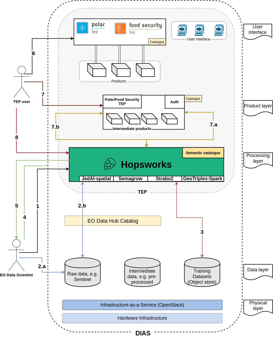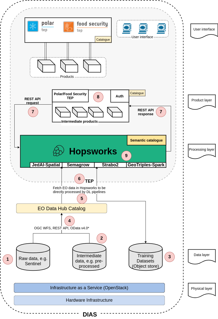We have tested these functionalities in two exercises which use data and queries from the Extreme Earth project, and finally, we have integrated Semagrow in Hopsworks as a means for providing a single access point to multiple data sources deployed in the Hopsworks platform.

System Description

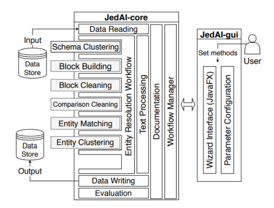
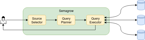
Semagrow receives a query through its endpoint, decomposes the query into several subqueries, issues the subqueries to the federated endpoints, combines the results accordingly, and presents the result to the user. In order to be able to extend Semagrow's capabilities to federated linked geospatial data, we developed novel techniques for federated geospatial linked data, and we have extended and re-engineered almost every component of Semagrow's architecture [4]. In the following figure, we illustrate the information flow in Semagrow, and the three major components that comprise Semagrow’s architecture:

In the remainder of the section, we will describe the current state of Semagrow, by discussing the improvements to each component in detail.

The first component of Semagrow is the source selector, which identifies which of the federated sources refer to which parts of the query. In particular, the goal for the source selector is to exclude as many redundant sources as possible, but without removing any source that contains necessary data for the evaluation of the query. Semagrow uses a sophisticated source selector that combines two mechanisms; one that targets thematic data and makes use of all the state-of-the-art source selection methods in the federated linked data literature; and a novel geospatial source selection mechanism that targets geospatial linked data specifically [5]. The idea behind this novel approach is to annotate all federated data sources with a bounding polygon that summarizes the spatial extent of the resources in each data source, and to use such a summary as an (additional) source selection criterion in order to reduce the set of sources that will be tested as potentially holding relevant data. This method can be useful in practice, because geospatial datasets are likely to be naturally divided in a canonical geographical grid (consider, for example, weather and climate data) or following administrative regions or, more generally, areas of responsibility (consider census data as an example).

The second component of Semagrow is the query planner, which uses the result of the source selector in order to construct an efficient query execution plan by arranging the order of the subqueries in an optimal way. Semagrow uses a dynamic-programming-based approach and exploits statistical information about each of the federated sources and a cost model for forming the optimal plan of a federated query. The effectiveness of the query planner is increased with the use of additional pushdown optimizations. Pushing the evaluation of some operations in the federated sources can be effective not only due to the reduction of the communication cost, but also because geospatial operations are computed faster by the remote GeoSPARQL endpoints; notice that, in general, a geospatial source maintains its own spatial index for evaluating geospatial relations. Finally, the query planner of Semagrow is able to process complex GeoSPARQL queries that were derived from the use cases of Extreme Earth [6]. These queries have complex characteristics (such as nested subqueries and negation in the form of “not exists” operation), and, to the best of our knowledge, cannot be processed by any other state-of-the-art federation engine.

The third component of Semagrow is the query executor, which evaluates the query execution plan, by providing a mechanism for issuing queries to the remote endpoints and an implementation of all GeoSPARQL operators that can appear in the plan. Apart from standard GeoSPARQL endpoints, Semagrow can support several non-SPARQL dataset servers through a series of executor plugins. We offer a plugin for communicating directly with PostGIS databases with shapefile data that contain geometric shapes exclusively. For implementing federated geospatial joins, Semagrow uses bind join with a filter pushdown (i.e., it fetches “left-hand” shapes to partially bind two-variable functions and pushes the filter to the “right-hand” endpoint). This approach is effective for standard spatial relations, but not for federated within-distance queries, i.e., for queries where the distance between two shapes from different sources has to be less than a specific distance. This happens because standard spatial relations can be answered very fast by the spatial indexes of the source endpoints, while the distance operator cannot. For speeding up within-distance queries, we offer an optimization which rewrites each subquery by inserting additional geospatial filters that filter out results that are too far away, but these additional filters use standard spatial relations (and can be executed fast by the source endpoints).

We mentioned that several parts of Semagrow rely on dataset metadata (e.g., the boundaries of the source endpoints for the geospatial selector). For this reason, we provide sevod-scraper, which is a tool that creates dataset metadata [7] from RDF dumps.

Extreme Earth Use Cases

The new version of Semagrow was tested and evaluated using data and queries derived from practical use cases in the context of Extreme Earth. In particular, we have used Semagrow in the following use cases: (a) linking land usage data with water availability data provided for the Food Security Use Case; and (b) linking land usage data with ground observations for the purpose of estimating crop type accuracy.

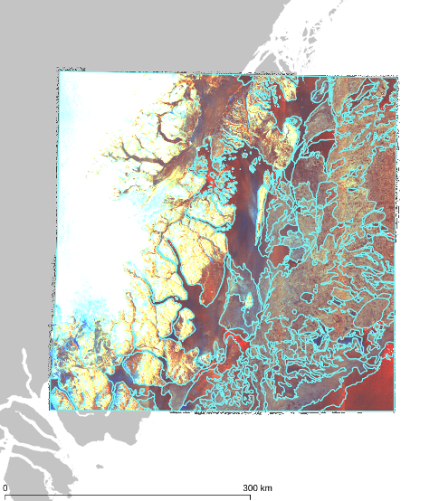
Food security is one of the most challenging issues of this century, mainly due to population growth, increased food consumption, and climate change. The goal is to minimize the risks of yield loss while making sure not to damage the available resources. Of great importance is the study of irrigation, which requires reliable water resources in the area being farmed. Considering the fact that a large portion of the world's freshwater is linked to snowfall and snow storage, a promising way for providing an indication of water availability for irrigation is to study the snow cover areas in conjunction with the field boundaries and their crop-type information. The queries that are most relevant for this analysis are spatial within queries, spatial intersection queries, and within-distance queries: that is, retrieving the land parcels with a given crop type that are within, intersecting, or within a given maximum distance (without requiring the exact distance) from any snow-covered area. Moreover, sometimes we need to reduce our focus either on a smaller polygonal area with given coordinates, or on a specific administrative region.

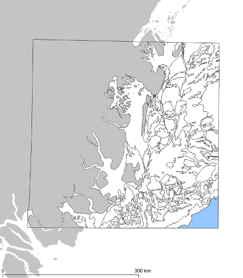
We have used Semagrow in an exercise based on the above use case as follows: We created a federation that consists of geospatial RDF data that cover Austria in three three data layers (i.e., snow, crop, and administrative data). In particular, we envisage that Austrian state governments publish crop datasets for their own area of responsibility; and a further (different) entity publishes a snow cover dataset that ignores state boundaries and publishes its datasets according to a geographical grid. 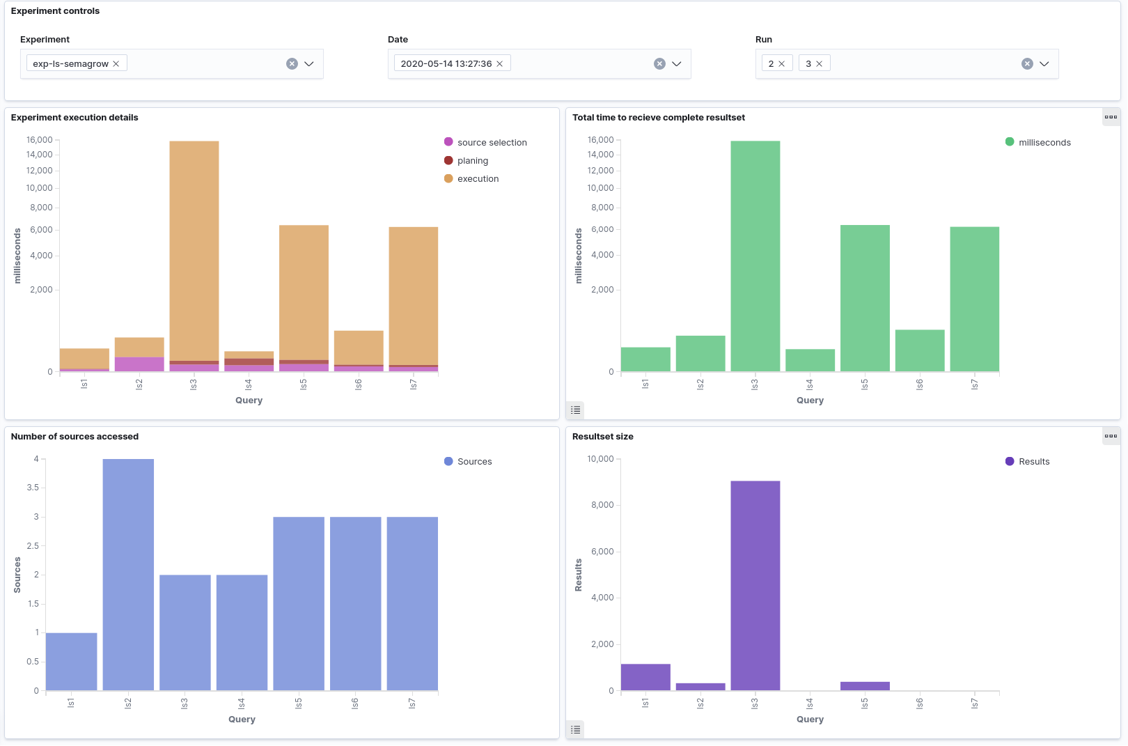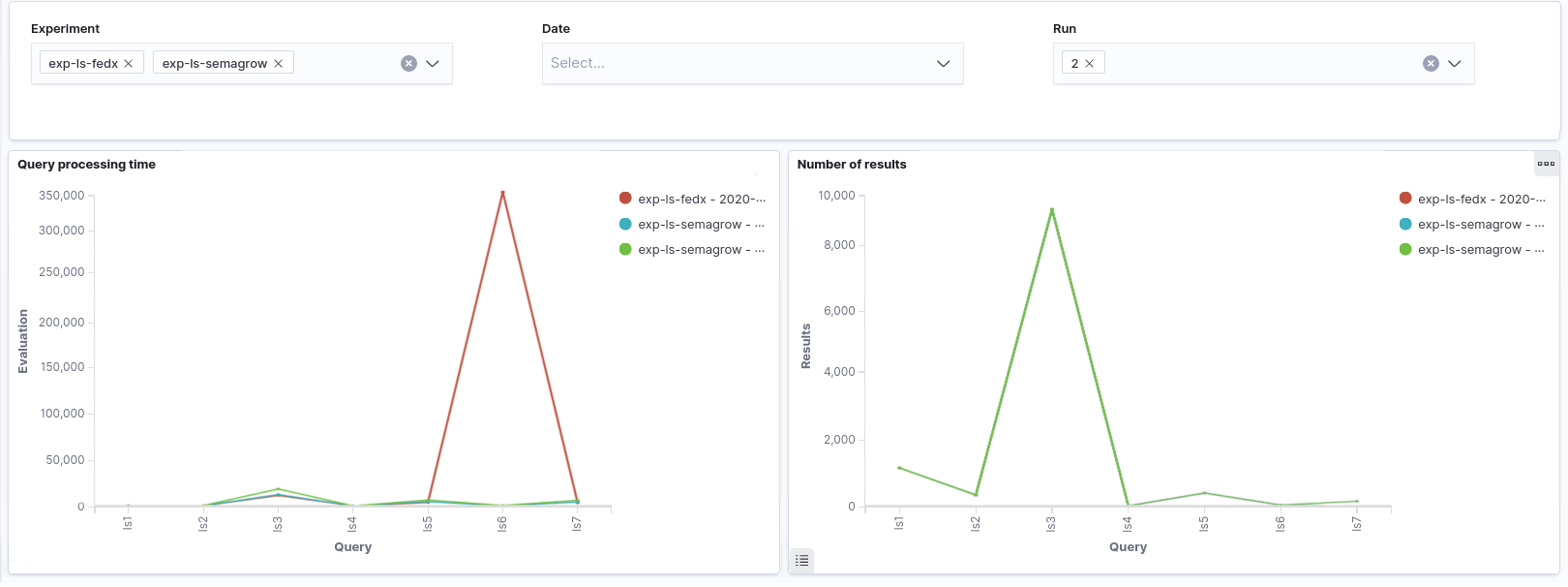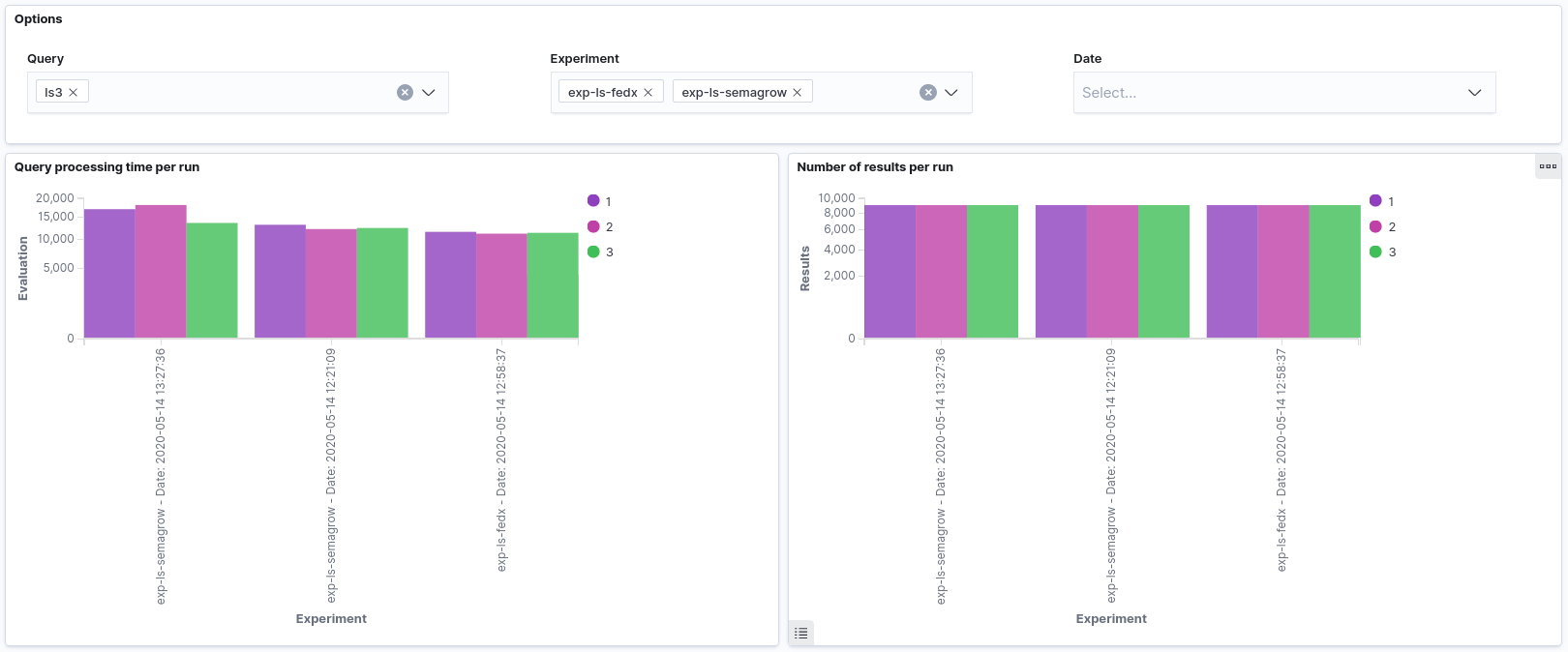Therefore, each federated endpoint contains data from a specific data layer and for a specific area (e.g., crop data of the state of Upper Austria). We used Strabo2 for serving the data. Since Semagrow is a standard GeoSPARQL endpoint, the results were able to be visualized in Sextant. In this series of experiments, we observed that the new version of Semagrow performs better than the old one, mainly due its source selector. Since the new source selector is aware both of the geospatial and thematic nature of the federated sources, it is able to effectively reduce the sources that appear in the query execution plan, and as a result to reduce the source queries issued by the query executor to the endpoints of the federation.

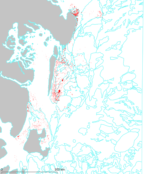
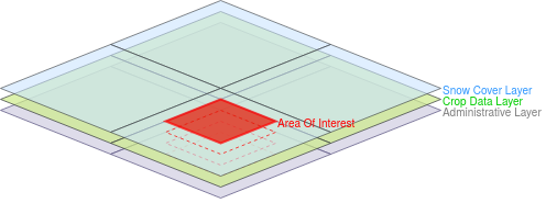
In the following figure, we illustrate a simplified version (4 snow, 4 crop, and 4 administrative sources, non-overlapping and perfectly aligned bounding polygons) of the above case. Assume that we want to retrieve all snow-covered crops within a specific area of interest shown in red. In this case, our source selection first prunes all administrative sources since they contain irrelevant thematic data; and then it prunes the sources that are disjoint from the area of interest since they contain irrelevant geospatial data. As a result, the query will be evaluated faster since the query execution plan will contain only 2 (of the total 12) sources.

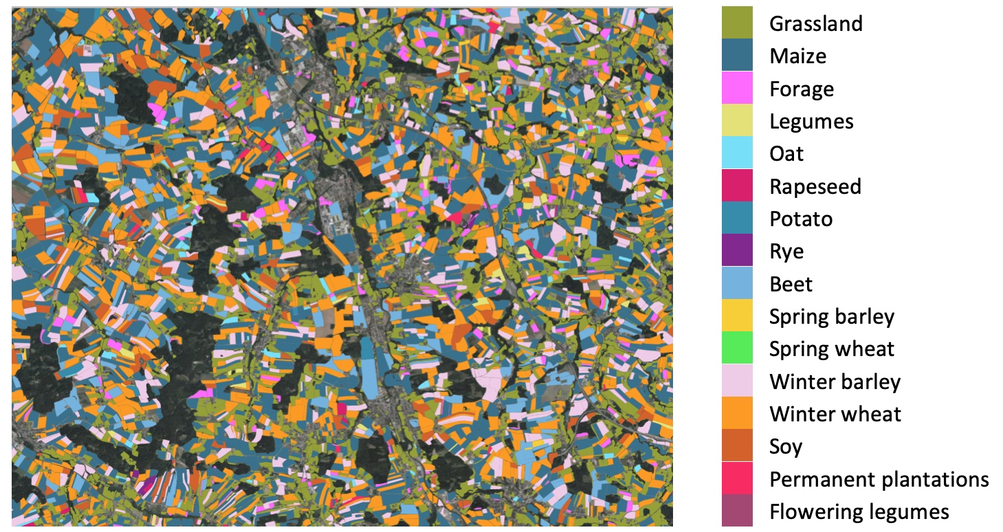
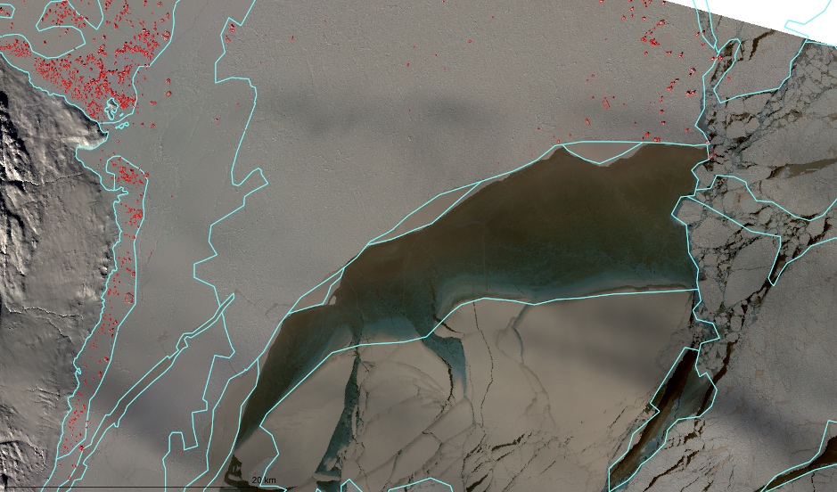
Detailed land usage data is crucial in many applications, ranging from formulating agricultural policy and monitoring its execution, to conducting research on climate change resilience and future food security. Land usage can be inferred from Earth Observation images or collected through self-declaration, but in either case it is important for such data to be validated against land surveys. Ground observations are geo-referenced to a point on the road adjacent to a field (and not inside a field), which is often ambiguous in agricultural areas with several adjacent parcels; further exacerbated by GPS accuracy. Therefore, we can estimate the error rate of the land usage data as follows: first, all ground observation is irrelevant to the analysis if it is more than 10 meters from any crop parcel. For the remaining ground observations, we find the nearest land parcel, and if the crop types match, the GPS point provides a positive validation; otherwise it provides a negative one. This process is challenging not only because it is computationally demanding (since it involves quadratic many distance calculations), but because the crop types between different datasets usually make use of different code names.

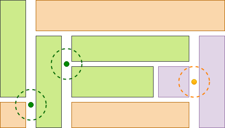
In the following figure, we illustrate 3 ground observations located in the roads adjacent to field parcels, used for crop-type validation of the field dataset. Notice that two of them (the green ones) provide a positive and the other one provides a negative validation.

We have used Semagrow for the task of the crop-data validation of the Austrian Land Parcel Identification System (INVEKOS), which contains the geo-locations of all crop parcels in Austria and the owners' self-declaration about the crops grown in each parcel. This dataset was validated using the EUROSTAT's Land Use and Cover Area frame Survey (LUCAS), which contains agro-environmental and soil data by field observation of geographically referenced points. Both datasets were transformed into RDF with GeoTriples, and were deployed in two separate Strabo2 endpoints. The new version of Semagrow completes the task very efficiently due to the federated within-distance optimizer; even though the queries of the task contain several complex characteristics (such as subqueries and negation), the bottleneck of the evaluation is the calculation of the within-distance operator. By disabling the optimization, the processing of the queryload would require several days, while with the optimization in place, the task reduces to several hours.

Conclusion

In this post we presented the new version of the Semagrow query federation engine, which was developed during the Extreme Earth project. Semagrow provides unified access to big linked geospatial data from multiple, possibly heterogeneous, geospatial data servers. All phases of the federated query processing (namely source selection, query planning and query execution) of Semagrow were extended, and Semagrow has been successfully integrated within Hopsworks. This new version of Semagrow was used and evaluated on data and queries from the use cases of the Extreme Earth project.

References

[1] Angelos Charalambidis, Antonis Troumpoukis, Stasinos Konstantopoulos: SemaGrow: optimizing federated SPARQL queries. In SEMANTICS 2015, Vienna, Austria, September 15-17, 2015

[2] Stasinos Konstantopoulos, Angelos Charalambidis, Giannis Mouchakis, Antonis Troumpoukis, Jürgen Jakobitsch, Vangelis Karkaletsis: Semantic Web Technologies and Big Data Infrastructures: SPARQL Federated Querying of Heterogeneous Big Data Stores. In ISWC 2016 (Posters & Demos), Kobe, Japan, October 17-21, 2016

[3] Athanasios Davvetas, Iraklis Klampanos, Spyros Andronopoulos, Giannis Mouchakis, Stasinos Konstantopoulos, Andreas Ikonomopoulos, Vangelis Karkaletsis: Big Data Processing and Semantic Web Technologies for Decision Making in Hazardous Substance Dispersion Emergencies. In ISWC 2017 (Posters, Demos & Industry Tracks), Vienna, Austria, October 21-57, 2017

[4] Antonis Troumpoukis, Nefeli Prokopaki-Kostopoulou, Giannis Mouchakis, Stasinos Konstantopoulos: Software for federating big linked geospatial data sources, version 2, Public Deliverable D3.8, Extreme Earth Project, 2021.

[5] Antonis Troumpoukis, Nefeli Prokopaki-Kostopoulou, Stasinos Konstantopoulos: A Geospatial Source Selector for Federated GeoSPARQL querying. Article in Preparation.

[6] Antonis Troumpoukis, Stasinos Konstantopoulos, Giannis Mouchakis, Nefeli Prokopaki-Kostopoulou, Claudia Paris, Lorenzo Bruzzone, Despina-Athanasia Pantazi, Manolis Koubarakis: GeoFedBench: A Benchmark for Federated GeoSPARQL Query Processors. In ISWC (Demos/Industry) 2020, Online, November 1-6, 2020

[7] Stasinos Konstantopoulos, Angelos Charalambidis, Antonis Troumpoukis, Giannis Mouchakis, Vangelis Karkaletsis: The Sevod Vocabulary for Dataset Descriptions for Federated Querying. In PROFILES@ISWC 2017, Vienna, Austria, October 21-57, 2017

Classifying sea ice satellite imagery - The workflow for the Polar Use Case

Identifying and investigating satellite imagery of sea ice is a complex -and in some cases frustrating- task for the sea ice analyst. As the seasons change, so do the reflectivity signals coming from the ice, meaning SAR imagery can look different from one month to the next. This is why MET Norway has dedicated sea ice analysts drawing our ice charts from the local knowledge built up and passed down through the years.

Automation of sea ice charting to reduce manual labour is an ultimate goal that has taken large footsteps in the right direction within the Extreme Earth project. As part of the Polar Use Case we have developed a workflow towards taking satellite imagery, transferring it to the Polar Thematic Exploitation Platform (Polar TEP) and classifying the image(s) based on algorithms developed by our partners. In this blog post we will give an outline of the workflow we have chosen to run with as the Extreme Earth Project comes to its conclusion.

The steps from Hopsworks to Polar TEP. The model is trained on Hopsworks, downloaded, docker container constructed and then the docker container is pushed to the Polar TEP docker registry before being made available on the web interface.

Firstly, we always assume that the model will be trained on Hopsworks (a data intensive AI platform). These deep learning and machine learning algorithms form the foundations for classification of satellite imagery, and have been trained using training data developed for the project. The training data in this case was mostly manually labeled satellite data, which teaches the machine learning model. Think of this process like the human brain, we take in information from the world around us (training data) and develop connections in the brain which help us to predict the outcome of a similar situation. For example, being taught to ride a bicycle, we are taught, we practice and then we don’t forget.

Secondly, we take the developed model and export it to disk as a zip file, from which, a docker container can be built. In simple terms, a docker container is simply a template that contains the model and the dependencies required to run the model. You could also sum it up by calling it a ‘software package’. The docker container can be made on any machine, even your own laptop at home, making it a useful tool for developers.

Once the docker container has been created, the ‘processor’ can be published to the Polar TEP web interface by accessing the Polar TEP development virtual machine (digital version of a physical computer). The docker container is pushed to the Polar TEP docker registry, making it available for viewing and use by the developer, who can then share the processor to all end users. The same docker container developed for use on Polar TEP could also be run on MET Norway’s post processing infrastructure.

An end user’s interaction with the platform and the hidden process of the processor.

For the end user, it is a simple procedure of selecting the satellite images they wish to process in the Polar TEP web interface and choosing the processor they want to classify the image(s). The result can then be downloaded and viewed in GIS software such as QGIS. In the example below, we can see an image that has been classified to show 4 classes, unknown, land, water, and ice, using the supervised VGG16 model developed by our partners at the University of Tromsø.

The QGIS interface showing a classified image with clear definition between water, ice and land.

The workflow presented here is now tried and tested with promising results. The Polar TEP platform has succeeded in providing an arena for scientists, developers and end users to share and exploit Copernicus big data. The platform has also offered a bridge between operations and research. These are two distinctively different groups with a history of un-synchronized co-operation in terms of using the same data format specifications and standards. In terms of operational use, models developed for the project are still deemed too immature, however, early results show promise for at least seasonal and or regional implementation. Due to the Extreme Earth project, we have come significantly closer to developing operational techniques which could be vetted by ice analysts.

KOBE: A Cloud-native Open Benchmarking Engine for Federated Query Processors

KOBE [1] is an open source benchmarking engine that leverages modern containerization and Cloud computing technologies (such as Docker and Kubernetes) in order to reproduce experiments in the context of federated GeoSPARQL query processing.

Introduction and Motivation

Federated query processors are systems that seamlessly integrate data from multiple remote dataset servers. More and more data providers choose to publish their datasets through public SPARQL endpoints, a situation which explains the growing interest in federated query processing technologies in the Linked-Data community. Several federation engines have been proposed (e.g., DARQ, SPLENDID, FedX, Semagrow, ANAPSID, CostFed, Odyssey) each with their own characteristics, strengths, and limitations. Naturally, consistent and reproducible benchmarking is a key enabler of the relevant research, as it allows these characteristics, strengths, and limitations to be studied and understood.

There are several benchmarks that aim to achieve this, but, similarly to the wider databases community, to release a benchmark amounts to releasing datasets, query workloads, and, at most, a benchmark-specific evaluation engine. However, reproducing and executing a benchmark with such a high-level description, presents several challenges to the experimenter:

• First, setting up an experiment requires a lot of effort, since it involves the deployment of many components: that is, several dataset servers and federators for running the queries and software to execute the query load.
• Second, more effort is needed for simulating real-life querying scenarios (such as experiments that take into account the network latency from the dataset servers to the federator).
• Finally, the experiment results should be presented in a useful and intuitive manner; again, this process is not trivial since it involves collecting logs from many components to come up with a meaningful result.

Based on our own experience with federated query processing research, we have been looking for ways to minimize the effort required and the uncertainty involved in replicating experimental setups from the federated querying literature. In particular, we were faced with the need of a tool that helps us in the task for conducting our experiments. For this reason, we have developed KOBE as a tool for executing our own experiments, but we find that it can be useful in both the benchmarking and linked data community.

Features

Features the KOBE benchmarking engine provides include:

• Automation of the various tasks: Setting up an federated querying experiment involves a lot of tedious tasks; i.e., the deployment, initialization of several components such as the dataset servers of the federation, the federator, and the software that executes the query load. KOBE reduces the time and effort of the experimenting process by providing an automation of these repetitive tasks.
• Reproducibility in different environments: Each component of the experiment is deployed in its own Docker container. Thus, KOBE allows for benchmark and experiment specifications to be reproduced in different environments and to produce comparable, consistent, and reliable results.
• Declarative specifications: All benchmarking components are specified using a declarative formalism that hides from the user the ugly details of provisioning and orchestrating. Thus, the KOBE user is concerned only about the queries to run, the datasets to use, and the engines to deploy.
• Simulating real-life scenarios: The characteristics of the computing infrastructure where a real-life data service is deployed and the quality network connection between the data service and the client [2] can affect the latency and throughput at which the federation engine receives data. KOBE allows defining experiments that simulate real-life scenarios by injecting network delays and latency limitations in each link between a dataset server and the federation engine.
• Results presentation: KOBE offers to the experimenter the ability to compare the performance of different setups of the same benchmark (e.g., different federators or data sources) and to draw conclusions for a specific setup by examining time measurements for each phase of the query processing and several other metrics. This is obtained by collecting logs from several benchmark components and a visualization using a WebUI.
• Extensibility: KOBE provides various extensibility opportunities and by design welcomes contributions from the community. In particular, KOBE supports the integration of new federators, dataset servers, and query evaluators.

System Description

KOBE consists of three main subsystems that control three aspects of the benchmarking process:

• The Deployment Subsystem, which is responsible for deploying, initializing, and orchestrating all components required by an experiment. components required by an experiment. This subsystem uses Kubernetes to handle the allocation of computational resources with a custom Kubernetes operator.
• The Networking Subsystem, which is responsible for connecting the different components of an experiment and for simulating network latency between the nodes of the federation as described by the benchmark. This subsystem uses Istio for controlling the network links through virtual proxies.
• The Logging Subsystem, which is responsible for collecting the logs produced by the several components (i.e, data sources, federators and evaluators), and for producing meaningful diagrams and graphs about the benchmarking process. This subsystem uses the EFK stack, a popular solution for a centralized, cluster-level logging environment in a Kubernetes cluster.

In the figure below, we illustrate the architecture and the individual components of an example experiment that contains a federation with three data sources:

Figure 1: Information flow through a KOBE deployment

The user edits the experimental configuration files and uses kobectl (the KOBE command-line client) to deploy and execute the benchmarking experiments, at a level that abstracts away from Kubernetes specifics. Experimental results are automatically collected and visualized using the EFK stack. The results of the experiment can be visualized by accessing the following dashboards.

Figure 2: Details of a specific experiment execution

The first dashboard (Figure 2) focuses on a specific experiment execution. It consists of four visualizations:

1. Time of each phase of the query processing for each query of the experiment.
2. Total time to receive the complete result set for each query of the experiment.
3. Number of sources accessed for each query of the experiment.
4. Number of returned results for each query of the experiment.

The first and the third visualizations are obtained from the logs of the federator engine; if such log messages do not exist these visualizations are empty. On the other hand, the second and the fourth visualizations are obtained from the logs of the evaluator, therefore they contain metrics in every experiment execution. All times are displayed in milliseconds. The exact metrics of each visualization can be also exported in a CSV file.

The remaining two dashboards can be used to draw comparisons between several experiment executions in order to directly compare different setups of a benchmark. The second dashboard (Figure 3) can be used for comparing several experiment executions. It consists of two visualizations:

1. Total time to receive the complete result set for each specified experiment execution.
2. Number of returned results for each specified experiment execution.

Figure 3: Comparison of experiment executions

These visualizations are obtained from the logs of the evaluator; all times are displayed in milliseconds; and, as previously, the exact metrics of each visualization can be exported in a CSV file. As in the first dashboard, each bar refers to a single query of the experiments presented.

Figure 4: Comparison of experiment ruins

The third dashboard (Figure 4) displays the same metrics as of the second dashboard. The difference here, though, is that we focus on a specific query and compare all runs of this query for several experiment executions. Contrary to the visualizations of the other two dashboards, each bar refers to a single experiment run, and all runs are grouped according to the experiment execution they belong to.

Extensibility and use in ExtremeEarth

KOBE provides various extensibility opportunities and by design welcomes contributions from the community. In particular, KOBE can be extended with respect to the database systems, federators, query evaluators and benchmarks that comprise an experiment. We currently provide specifications for two dataset servers, namely for Virtuoso and Strabo2; and for two federators, FedX and Semagrow. These systems have very different requirements in terms of deployment, providing strong evidence that extending the list of supported systems will be straightforward.

We have used KOBE extensively during ExtremeEarth as a tool for the benchmarking tasks of the linked data tools the project. In particular, we have extended KOBE with three new benchmarks that target big linked geospatial data specifically. These benchmarks are Geographica 2 (for single node linked geospatial stores), Geographica 3 CL (for distributed big linked geospatial stores), and GeoFedBench (for federated linked geospatial data).

• Geographica 2 [3] is the second iteration of the Geographica benchmark and contains big real world datasets, new tests and queries that reveal the scalability of single node linked geospatial stores.
• Geographica 3 CL [4] is based on synthetic datasets and queries that scale well beyond the sizes of Geographica 2 (hundreds of TBs instead of hundreds of GBs), and it includes a distributed synthetic data generator for deploying the datasets into multi-node HDFS-derivative clusters (such as Hopsworks).
• GeoFedBench is a benchmark for federated linked geospatial data processors, and it is both informative and realistic; not only it challenges all phases of federated querying but also it comes from practical scenarios obtained from the use cases of ExtremeEarth.

Apart from the benchmarks that target geospatial data and were developed in the context of ExtremeEarth, we provide benchmark specifications for existing linked data benchmarks (such as LUBM, FedBench, LargeRDFBench, OPFBench [7]).

For more information for how to use and extend KOBE, please visit the KOBE user guide. This guide contains step-by-step instructions and HOW-TOs for installing and uninstalling KOBE; for performing an experiment and viewing its results, for creating new benchmarks and experiments; for tuning network settings; for extending it with new data federations, new dataset servers and new query evaluators; and finally for providing metric support and adding new evaluation metrics.

Conclusions

In this blog post, we have presented KOBE, an open-source benchmarking engine that reads declarative benchmark and experiment definitions and uses modern containerization and Cloud computing technologies for automating the process of deployment, initialization, and experiment execution processes. The engine offers simulation of realistic endpoint delays and provides collection of logs and visualization of the experiment results using a WebUI. We have used KOBE for conducting our experiments in ExtremeEarth.

References

[1] Charalampos Kostopoulos, Giannis Mouchakis, Antonis Troumpoukis, Nefeli Prokopaki- Kostopoulou, Angelos Charalambidis, and Stasinos Konstantopoulos. KOBE: Cloud-Native Open Benchmarking Engine for Federated Query Processors. In ESWC 2021, 6-10 June, held on-line, 2021. [nominated for best resource paper award]
[2] Pierre-Yves Vandenbussche, Jürgen Umbrich, Luca Matteis, Aidan Hogan, and Carlos Buil Aranda. SPARQLES: Monitoring public SPARQL endpoints. Semantic Web 8(6): 1049-1065, 2017
[3] Theofilos Ioannidis, George Garbis, Kostis Kyzirakos, Konstantina Bereta, and Manolis Koubarakis. Evaluating geospatial RDF stores using the benchmark Geographica 2. J. Data Semant., 10(3-4):189-228, 2021.
[4] Antonis Troumpoukis, Nefeli Prokopaki-Kostopoulou, Giannis Mouchakis, Babis Kostopoulos, Angelos Charalambidis, Stasinos Konstantopoulos, Dimitris Bilidas, Theofilos Ioannidis, Michail Mitsios, George Smyris and Manolis Koubarakis .Evaluation framework for linked geospatial data systems. Public Deliverable 3.5, ExtremeEarth Project, December 2021.
[5] Antonis Troumpoukis, Stasinos Konstantopoulos, Giannis Mouchakis, Nefeli Prokopaki-Kostopoulou, Claudia Paris, Lorenzo Bruzzone, Despina-Athanasia Pantazi, and Manolis Koubarakis: GeoFedBench: A Benchmark for Federated GeoSPARQL Query Processors. In ISWC (Demos/Industry) 2020, 2-6 November, held on-line, 2020
[6] Antonis Troumpoukis, Angelos Charalambidis, Giannis Mouchakis, Stasinos Konstantopoulos, Ronald Siebes, Victor de Boer, Stian Soiland-Reyes, and Daniela Digles. Developing a Benchmark Suite for Semantic Web Data from Existing Workflows. In BLINK@ISWC 2016, Kobe, Japan, October 18, 2016.